IRSIM version 9.7 Tutorial

Table of Contents

IRSIM, the switch-level simulator

Transistor state
Logic value
Transistion events

Creating a .sim file
Starting IRSIM
Running IRSIM
Using the analyzer window

Print the waveforms to a PostScript file
Zooming and Scrolling Changing the base of nodes Changing the order of the nodes
Finding the time of an event

Vectors
Clock Definition
Scheduled events
Tristate values
Simulation settings
Quitting IRSIM
Automation through command files
IRSIM essential commands
Converting Verilog testbenches to IRSIM
Tutorial History

IRSIM, the switch-level simulator

This is a simple online tutorial on IRSIM. It is not meant to replace the IRSIM manual which contains much more information. The IRSIM online manual is currently available at OpenCircuitDesign.com:

http://opencircuitdesign.com/irsim

IRSIM is a switch-level simulator, in the sense it models the circuit at the level of transistors. The transistors are modeled as switches, ignoring most of the higher-order and analog properties of the devices and instead treating each device as an ideal on-or-off connection. A switch-level simulator considers three important aspects of digital circuit behavior:

1. Transistor state (on or off)
2. Logic value (high or low)
3. Transistion events (from one logic value to another)

Transistor state

The original version of IRSIM used true switch models. A later refinement introduced the linear model, which captures the first-order deviation of real transistors from an ideal switch by modeling each device with two states: high resistance (path from source to drain), and low resistance. In essentially all CMOS processes, the "off" or high resistance state is effectively the same as the ideal case; it's the "on" or low resistance state that deviates the most from the ideal switch. By using the linear model, IRSIM can more accurately reflect differences between different transistor types, gate rise and fall times, and different fabrication processes.

Logic value

IRSIM treats all voltages in a circuit as being one of three symbolic values:

1. high, h, 1
2. low, l, 0
3. indeterminate or unknown, x

This simplification prevents IRSIM from having to know what is the actual voltage powering the circuit, instead dealing with a voltage value "normalized" to 1. The linear model works with these normalized voltages and will even compute how charge sharing generates an intermediate (normalized) voltage, but in the end every node in the circuit must resolve to one of the three values.

Transistion events

In addition to the simplified modeling of devices, IRSIM is also unlike a true circuit simulator such as SPICE in that it treats the circuit as a cascade of events. Every switch-model transistor has a controlling gate and a source-to-drain path that is either on or off. When the transistor switch is "off", the transistor source and drain nodes belong to two separate paths which may have independent states. When the transistor switch is "on", the transistor source and drain nodes are combined into a single path, which can only have one state. The change in state of a gate is an event that causes IRSIM to re-evaluate the paths around that transistor's source and drain. In a well-constructed circuit, every path should be driven by a single value, high or low. In a some circuits, a path may be driven by multiple values (bus contention) or it may be electrically isolated (tri-state). These conditions are not necessarily errors! IRSIM even has ways of coping with such conditions, but the behavior is not well modeled. Circuit design that create these conditions are better suited to full analog simulation than to switch-level simulation.

Creating a .sim file

Typically we will use a schematic capture editor (such as XCircuit) to create a circuit for analysis, or we will use a layout editor (such as Magic) to create a circuit and then extract the circuit netlist and analyze the result with IRSIM. We can also use a digital synthesis flow to generate a circuit from verilog, place and route it, then use IRSIM to confirm that the synthesized circuit matches the original behavioral description. Hence typically we do not create a .sim circuit description manually, as is described below. Manually creating a circuit netlist description (.sim file) for IRSIM is really only useful for tutorial purposes, such as this one.

All the files IRSIM uses are just text files that contain information about a circuit and its behavior. The circuit netlist files have the extension .sim. The first time you use IRSIM, you will probably want to create the .sim file yourself using your favorite text editor. The following file, though, can also be generated from XCircuit or any schematic capture system (you can download the XCircuit PostScript by clicking on the circuit image below, then generate the .sim file from the XCircuit menu "Netlist->Write sim"). The resulting file irsim_logic.sim can also be obtained by clicking on the link in this sentence.

Below is a CMOS circuit to implement the 2-input logic function

out = (!a . !b) + !c

where !a means the inverse (Boolean NOT) of a, "." is the Boolean logic function AND, and "+" is the Boolean logic function OR. The first step in creating a .sim file for this circuit is to label all the nodes. Label power Vdd and ground Gnd. IRSIM is not case sensitive so "vdd" and "gnd" will work interchangeably. You can label the other nodes anyway you want. Use any method you wish. For the circuit above, the inputs are labeled a, b, c; and the output node is labeled out. Other internal nodes are arbitrarily labeled n1 and n2. When using IRSIM, it is helpful to have the labeled circuit schematic available so that you know the names of the nodes that you want to probe. The irsim_logic.sim file for the above circuit is shown below.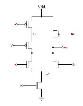

line     text 1 |units: 100 tech: scmos 2 | 3 |type gate source drain length width 4 |---- ---- ------ ----- ------ ----- 5 p a vdd n1 2 4 6 p b n1 out 2 4 7 p c vdd out 2 4 8 9 n a out n2 2 4 10 n b out n2 2 4 11 n c n2 gnd 2 4

The first four lines are comments. Any line that begins with the vertical bar '|' is a comment. This first line says that the technology used is scalable cmos, with a process "lambda" (1/2 minimum feature size) of 1 micron (the number "units" is in "centimicrons", or units of 1/100 micron, so 100 centimicrons is 1 micron). IRSIM will parse this line and use the information to check if the file contents match the parameter file it loaded on startup.

Transistors are specified as follows:

type gate source drain length width

where type is p for pmos and n for nmos. The gate, source, and drain refer to the terminals of the transister. This is why you need a labeled circuit schematic to create a .sim file by hand. It is important that you get the connections correct. The length and width of the transistor are both in microns.

The first transistor specified in the example above is the top-left pmos transistor in the corresponding schematic. Study the rest of the IRSIM file and the circuit. It is easy to see how the two match. You can also enter in resistors and capacitors. See the IRSIM manual for the proper format to create these elements. Considering just transistors, you are now ready to run IRSIM.

Starting IRSIM

At the unix prompt type

irsim scmos100.prm irsim_logic.sim

where irsim_logic.sim is the simulation file and scmos100.prm is a standard parameter file for a 2.0 micron process technology.

If you have the Tcl/Tk-based IRSIM version 9.7, you will get a console window with diagnostic output in blue, error output in red, and the Tcl prompt in brown. In the non-Tcl version, you will get the prompt

IRSIM>

in the terminal window. This tutorial will normally assume the use of the Tcl/Tk-based IRSIM, with deviations from the non-interpreter-based version noted. IRSIM will tell you how many transistors you have and then display the Tcl prompt shown below (with or without additional information, such as the current working directory and interpreter line history number:

%

Running IRSIM

You can enter in commands interactively or you can run a script. Scripts are just text files containing commands that are exactly what you would type in at the IRSIM prompt (see section 3.3 below). Here is an example IRSIM session. The "%" prompt precedes commands that were entered interactively. Text in blue is what is output from IRSIM.

% stepsize 50

The basic idea of IRSIM is that you tell it which nodes to pull high, which nodes to pull low, which nodes to tristate, and then you tell IRSIM to run the simulation for a certain period of time. This period of time is the stepsize. The above command tells IRSIM that the stepsize is 50ns. The default stepsize is 10 nanoseconds.

% h vdd
% l gnd

Because not all power supplies are so obviously labeled, it is necessary to provide power to your circuit by declaring the power supply ("vdd") to be logic high and ground ("gnd") to be logic low. This may seem trivial, but the simulation won't work without it.

% w out c b a

The command 'w' tells IRSIM to watch the following nodes. So the above command tells it to watch the nodes out, c, b, and a. IRSIM displays the nodes in the reverse order in the above command. Therefore the output order will be a b c out. This is just a matter of personal preference though. Enter in the nodes in any order you like.

% d

d displays all the nodes that are being watched. You can also enter in something like 'd a b' which tells IRSIM to only display nodes a and b

a=X b=X c=X out=X
time = 0.000ns

at time zero, the values of the nodes are all undefined

% l a b c

The l command forces the nodes to a logic low value of 0 The above command sets nodes a b and c to logic 0

% d
a=X b=X c=X out=X
time = 0.000ns

Note from the above an important feature of IRSIM: Changes to nodes are scheduled events and are not immediately applied to the circuit! So, to see the result of our "l" command, we must do:

% s

s tells IRSIM to simulate for a certain period of time previously defined by the stepsize command. The default value is 100 ns, but we set it to 50ns above.

a=0 b=0 c=0 out=1
time = 50.000ns

IRSIM displays the values of the nodes after each step because of the previous d command. The current time is also displayed. Note that time = 50 ns. This is the current simulation time now.

% h c

h sets the following nodes to a logic high value. Therefore the above command sets node c to logic 1.

% s
a=0 b=0 c=1 out=1
time = 100.000ns

step again:

% h b
% s
a=0 b=1 c=1 out=0
time = 150.000ns

% path out
critical path for last transition of out:
   b -> 1 @ 100.000ns , node was an input
   out -> 0 @ 100.001ns (0.001ns)

The path command shows the critical path for the last transition of a node. The output shows that an input node 'b' changed to logic 1 at time = 100 ns. The node 'out' then transitioned low at time = 100.001 ns. Therefore it took 1 ps to go from high to low for the given input changes. If this transition time seems rather low, it should! There is no parasitic capacitance information in the .sim file, so there is no information from which IRSIM can estimate a real gate delay. Thus, IRSIM uses its minimum delay of 1 internal unit for a gate delay. The command:

% unitdelay 0.1

would increase the unit gate delay from 1ps to 100ps, for example. However, this tutorial is not particularly concerned with the accuracy with which IRSIM models a specific process. You can look back at previous commands to verify that the stated critical path transition is indeed what happened. Sometimes you may want to find out what the worst case Tplh (time from input low to output high) or Tphl (time from input high to output low) is. The path command helps you find this number. You do this by setting the circuit to some state and then force inputs to change that will cause a transition at the output. Some intelligence is required to figure out what the worst state is and what combination of input changes will cause the slowest output transition. If you have a long list of inputs, it can be tiresome to keep using the l and h commands to set the logic values. The 'vector' command lets you group inputs together so that you can set them all quickly

% vector in a b c

The above command tells IRSIM to group the nodes a b and c into a vector called 'in'

% setvector in 000
000

This command tells IRSIM to set the vector in to (binary) 000 (node that versions of IRSIM prior to 9.7 used the "set" command, which has been changed in 9.7 because "set" has a different meaning to the Tcl interpreter language). Therefore, node a = 0, node b = 0, and node c = 0. The following commands demonstrate how you can create a truth table using the vector 'in'. Note that you can do this much faster this way than by using the commands l and h.

% s
a=0 b=0 c=0 out=1
time = 200.0ns
% setvector in 001
% s
a=0 b=0 c=1 out=1
time = 250.0ns
% setvector in 010
% s
a=0 b=1 c=0 out=1
time = 300.0ns
% setvector in 011
% s
a=0 b=1 c=1 out=0
time = 350.0ns
% setvector in 100
% s
a=1 b=0 c=0 out=1
time = 400.0ns
% setvector in 101
% s
a=1 b=0 c=1 out=0
time = 450.0ns
% setvector in 110
% s
a=1 b=1 c=0 out=1
time = 500.0ns
% setvector in 111
% s
a=1 b=1 c=1 out=0
time = 550.0ns

Because the Tcl version of IRSIM is based in an interpreter, the command sequence above can be reduced to the following Tcl code:

set vlist {000 001 010 011 100 101 110 111}
foreach vec $vlist {setvector in $vec ; s}

IRSIM has a built in graphical logic analyzer which lets you view waveforms. The 'analyzer' command sets up the analyzer window

% analyzer a b c out

This tells IRSIM to display the nodes a b c and out in the analyzer window

Using the analyzer window

Go ahead and experiment with the analyzer window. It's pretty easy to use. Here are some of the things that you can do.

Print the waveforms to a PostScript file

Go to the 'Print' menu and select 'File'. You will be asked for a filename. The result is a PostScript file which can be sent to a printer or viewed with a PostScript interpreter such as ghostview (gv).

Zooming and Scrolling

You can set the width and position of the view from the slider and buttons on the bottom, or you can use the menus. Use the 'Zoom' menu to zoom in and out or set the view to encompass the entire simulation.

The best way to get a feel for the slider on the bottom is to play with it. Grabbing and dragging the left mouse button moves the view forward or backward in time. Grabbing and dragging with the right mouse button on the slider expands the view or shortens the view to the right or left depending on where you click.

The left-most "target circle" button expands the view to encompass the entire simulation, just like choosing the button "Zoom->Full" from the menu. The double-left-arrow button moves to the start of the simulation, and the double-right-arrow buttons moves to the end of the simulation. The single-left-arrow button scrolls back one step, and the single-right-arrow scrolls forward one step. The scroll step size can be changed from the menu item Window->Scroll Step. The same scrolling action happens if you type the Left or Right arrow keyboard keys while the mouse pointer is in the display window.

Changing the numerical representation of nodes

Single nodes are always represented in the analyzer diplay as a signal graph drawn between low and high values, with infinite slope at transition points, and as a cross-hatch pattern when undefined. Vectors, on the other hand, may take on a number of different notations. By default, vectors are presented in binary notation, but vectors of more than 8 bits in length are presented in unsigned decimal notation. To change the representation, select the trace by clicking on the trace name. Then, go to the menu item "Base->", and select the type of representation from the list of checkboxes. Available representations are binary, octal, hexidecimal, signed integer, and unsigned integer. It is also possible to change the representation from the command line, or from a script, using the command "base set trace_name" followed by one of the style names mentioned above.

Undefined nodes are handled differently according to the base. In binary notation, every node in the vector is represented by its own character, so there is no ambiguity. In octal and hexidecimal notation, groups of bits (3 and 4, respectively) are represented by a single character. If any one of those bits is undefined, the character for that group of bits will be displayed as undefined. In signed and unsigned decimal notation, the relationship of decimal characters to bits is not N:1, and so any undefined bits in the vector will cause the entire vector value to be displayed as "???".

Changing the order of the nodes

If you don't like the order that the nodes are displayed, you can type the command, e.g.,

% trace move out c

to swap the traces "out" and "c". Everything that can be done to the GUI view is available as a command-line command. In addition to the "trace" command, the GUI can be queried and manipulated by the commands "simtime", "base", "marker", "print", and "zoom".

The special menu item "Window->Manage Traces" creates a pop-up listbox window that allows one to select which nodes and vectors to display or not to display from a list of all defined nodes and vectors. The display is divided up into four boxes labeled "Nodes", "Nodes in Analyzer", "Vectors", and "Vectors in Analyzer". The lists "Nodes" and "Vectors" show all of the nodes and vectors, respectively, that are not in the analyzer display. Clicking on a node or vector in one of these lists will create a trace in the analyzer window, while clicking on a node or vector in the "Nodes in Analyzer" and "Vectors in Analyzer" list will remove it from the analyzer.

Finding the time of an event

You can click the left mouse button inside the analyzer window where the waveforms are to get a vertical line. The time where this vertical line is is displayed above, and the instantaneous value of each signal on the display is printed to the right of the traces. This is useful if you want to find out when a rising edge occurs. The resolution is best when you are zoomed in.

Vectors

Since nodes typically are grouped into vectors, it is usually easier to look at N-bit quantities as single vector entities. The following commands can be used to define vectors and display them.

% vector name node1 node2 ...

define a new vector called name consisting of the list of nodes

% d name

display a vector as an array of bits

% ana name

add vector name to the waveform viewer

% setvector name value

set the bits of vector name using the binary string value To set a vector to a hexadecimal number, use:

% setvector name 0xhexstring

For instance, you can now say:

% setvector Va 0xff

if Va is an 8-bit (or larger) vector, instead of

% setvector Va 11111111.

The prefix 0x says that what follows is a hex constant. Likewise, IRSIM understands prefixes "0b" for binary (which is the same as having no prefix), "0d" for decimal, "0o" for octal, and also accepts "0h" for hexidecimal. Returning to the original example, we can refine the Tcl script even further by using decimal notation and applying simple arithmetic from Tcl, reducing the simulation to a single command line:

% for {set i 0} {$i < 8} {incr i} {setvector in 0d$i ; s}

A useful shortcut to define arrays as long lists of nodes is to have the nodes in numerical order, in which case a Verilog-like vector notation may be used:

% vector M M<8:1>

The above construction is only possible if nodes M<1> through M<8> exist and M<8:1> itself is not the name of a single node. Note that one may specify either M<8:1> or M<1:8>; in the first case, M<1> is the least significant bit (lsb) of the vector, and in the second case, M<1> is the most significant bit (msb). Note that the vector does not have to be defined by any specific delimiter (e.g., angle brackets). It is equally valid to write vector notation for a set of nodes defined simply as, for instance, M1, M2, etc.:

% vector M M8:1

Negative numbers can be represented in the decimal notation by putting the negative sign in front of the "0d". Negative numbers will be calculated according to 2's complement notation and the bit length of the vector. From the example above:

% vector M M8:1
% setvector M -0d1
% query M
255
% assert M
A = 11111111

You will note from the above example that while vectors may be set as negative numbers, they will never be reported as negative numbers by the "query" command (which, by the way, returns the negative number "-1" to indicate an error, such as an undefined or partially undefined vector). The analyzer is capable of displaying numbers in both signed and unsigned decimal notation by setting the base of the trace appropriately.

Clock Definition

The standard clock definition is shown below:

% vector CLOCK CLK _CLK
% clock CLOCK 01 10

The first line defines CLOCK to be a vector of two signals: CLK and _CLK. These signals are defined as globals in the file. The second line states that a single cycle of the clock consists of setting the vector first to 01 and then to 10. Once this clock is defined, you can run the simulation for a clock step by saying:

% c

The following runs the simulation for 10 cycles:

% c 10

The following runs for a single clock phase, stepping through the sequence of values defined for a clock:

% p

Scheduled events

The "clock" statement is very limited in usefulness, as it forces all input changes to be made at clock boundaries or, with considerably less succinctness, on clock phase transitions. Setting up a simulation to drive a circuit with multiple clocks at different periods is a truly painful task! IRSIM version 9.7 defines the commands "at" and "every". These commands allow a completely different method of simulating, in which the simulation inputs are set up first by scheduling, then the simulator run without further input. Again, going back to the original example, the same simulation can be defined in the following way:

set i 0
every 200 {setvector in 0d$i ; d ; incr i}
s 1200

In the first line, we set a Tcl variable "i" to zero. Then, we schedule a procedure to occur every 200 nanoseconds during the simulation. This procedure consists of three IRSIM statements:

1. "setvector" sets the new value of "in" to be equal to the (binary-converted) value of Tcl variable "i"
2. "d" displays the values on the watchlist
3. "incr i" increments the Tcl variable "i" by 1.

Following the scheduling statement, the simulator is run for 1200 nanoseconds. Every 200 nanoseconds, the defined procedure is executed. Because we used the "every" statement, after every execution, the procedure is rescheduled 200 nanoseconds in the simulation's future.

The "every" and "at" statements are especially useful, as they correspond very closely to verilog "always" and "#" commands. Note, however that verilog's "#" defines a delay from the previous event, whereas IRSIM's "at" command is specified in absolute time.

Events can be scheduled not only in absolute or relative time, but also in response to event changes. The commands "when" and "whenever" have a similar syntax to the "assertWhen" command, but are followed by a procedure to execute at the transition specified by the first two arguments. The first argument is a node name (vectors are not supported), and the second the value at the end of the transistion you want to trigger the procedure. In the following example:

when in0 h {h reset ; at +100 {l reset}}

On the next occurence of the transition of node in0 from low to high, the procedure will execute, forcing the signal reset high for 100ps. The procedure specified by when will execute once and only once. For a recurrent procedure that executes on every transistion of a signal, use the whenever command, which has a syntax exactly like when but reschedules the event after every execution. The "whenever" procedure works exactly like the verilog procedural block "@(posedge signal) begin ... end" (or negedge). Multiple conditions on more than one node (e.g., "in0 high AND in1 low" are not supported (which explains why you can't pass a vector name to the when and whenever commands). Multiple edges for a single node can be specified by concatenating edge types. For example,

whenever in0 hl {puts stdout [query in0]}

will print the value of node in0 on every transition low-to-high or high-to-low.

As with the every and at commands, the non-Tcl version of IRSIM can execute only IRSIM commands in the procedure, while the Tcl version may use arbitrarily complex procedures, including conditionals. The following piece of code simulates a VCO (voltage controlled oscillator):

	whenever reload h {
	   catch {every cancel $ev1}
	   set tp [expr {100 + 20 * [query var]}]
	   set ev1 [every $tp {toggle vco_output}]
	}
	

This piece of code assumes that there is a signal "vco_output" representing the output of the VCO, and a vector called "var" that represents a (digital) tuning input to the VCO. It also assumes that the signal reload is set high by the circuit to indicate that the tuning has changed. Whenever this happens, IRSIM evaluates the frequency of the VCO based on an equation (presumably derived from an analog simulation of the VCO circuit), and sets up the vco_output signal to toggle at that frequency.

Only one callback procedure can be specified for a single node using when or whenever. You can specify different actions at different edges. The following effectively copies the value of nodeA to nodeB:

	whenever clock hl {
	   if {[query clock] == 1} {
	      h clockcopy
	   } else {
	      l clockcopy
	   }
	}
	

A different command is used to break a simulation when a specific node or vector changes state. This is the "stop" command, and is used simply by stating:

stop node|vector

which will set a breakpoint at any transistion or change in the specified node or vector. If the simulation is in the middle of executing an "s" (step) or "c" (clock) command when the breakpoint condition is encountered, the simulation will stop.

Tristate values

You have seen the commands 'l' and 'h' to set nodes to logic 0 or logic 1. The 'x' command will effectively put a node into tristate. It does this by taking the node off the input list. It is unfortunate that IRSIM uses the command 'x' since unknown values are displayed as 'X' in the output. Just remember that the command 'u' drives the value of a node to "unknown", or 'X', while the command 'x' stops driving the value of a node altogether. The following is an example of using the x tristate command

% x bus

puts the node bus into tristate. An application of this is simulating a register. Assume you have a one bit register that is connected to a line called bus and is operated as follows. To write a value in your register, you need to drive the value onto the bus and then set a control line write to high. To read the register, you first need to stop driving the bus. Then set a control line read to high. The IRSIM commands you need to issue are shown below (note that the use of ";#" for comments is valid Tcl syntax).

%	l read write	;# set read and write control lines low
%	h bus	;# let's write a 1 into the register
%	s	;# step
%	h write	;# write into the register
%	s
%	l write	;# stop writing
%	s
%	l bus	;# set bus to 0 so we can see the bus
		;# transition from 0 to 1 when we read
		;# the register
%	s
%	x bus	;# stop driving the bus so we don't get
		;# bus contention when we read the
		;# register
%	s
%	h read	;# read the register; you should see a
		;# 0 to 1 transition

IRSIM lets you keep a log of your commands and the outputs. To start recording, type

% logfile anyfilename

Anything that you see in IRSIM from now on will be into the file 'anyfilename' When you're done recording, type the following.

% logfile

Simulation settings

Unit gate delays, node decay, and node contention

Every simulator is affected by various options and settings. Some of these are process-dependent, and appear in the parameter (".prm") file. The values in this file are fixed; if you know what process your circuit will be fabricated in, then use the parameter file for that process. There should be no need to change any values in the parameter file. If you don't know what process the circuit is targeted for, then don't worry; in a switch-level simulator, transistors are more or less ideal devices, and don't change properties much from process to process. You can likely simulate any circuit with any parameter file. If the circuit uses "standard" CMOS that does not depend on charge sharing, pass-gates, or similar circuits that are dependent upon characteristics of a transistor beyond the ideal switch, you are nearly guaranteed a reasonable simulation.

There are, however, a few simulation parameters that are not specifically related to process parameters, but which affect a simulation. If you are forced to use these parameters to get a simulation to work, be warned that IRSIM is only going to give you a result that indicates whether the circuit is functionally correct. To ensure that such a circuit is safe from glitches and other problems, it should be simulated with SPICE, over all process corners. Often, IRSIM is best used in conjunction with SPICE and/or mixed-mode simulators. IRSIM is the quick-and-dirty simulator that ensures that a circuit design is functionally correct, or in the case of synthesized logic, that the routed, extracted layout is functionally correct. Often it suffices to run a simple SPICE simulation to ensure that the circuit is free from hold-time violations, glitches, and other timing errors, while IRSIM can be used to quickly test an exhaustive set of test patterns, where a full SPICE simulation would take a prohibitively long time.

We have already mentioned the unit gate delay, set by the unitdelay command. Without knowledge of source and drain sizes and parasitic capacitances to the substrate, IRSIM has no way of correctly guessing the charging and discharging times at a node, and will set them to the minimum time step. The minimum time step is set very small to account for fast fabrication processes, and is likely not to be realistic in most cases.

Circuits that hold values on an electrically isolated node and then expect the charge on this node to set a value on a different node through charge sharing are inherently "dangerous" in the sense that they are highly dependent on process parameters and should not be expected to simulate correctly using a simple switch-level simulator. That said, however, one such circuit is the dynamic RAM memory cell, whose use is ubiquitous. If you can confirm through SPICE simulation (as described above) that the circuit is error-free, IRSIM will gladly run a fast simulation of such a circuit. IRSIM will normally assume that a voltage held on an electrically-isolated node is held there forever. But, one may want to catch problems that occur when a node is held in isolation too long without being refreshed. By setting the decay parameter to a (conservative!) estimate of the decay time due to leakage, IRSIM can catch instances where a circuit may have been designed with too little margin for error. The command is

% decay 100

to set a decay time of 100ns. After a node has been isolated from any driving voltages for 100ns, its value will be set to "X" (unknown).

One of the more important settings is set by the "settle" command. The problem solved by the "settle" time parameter is quite common and is probably the most likely cause for simulation failure in IRSIM. The problem arises when two driving voltages with different logic values attempt to drive the value of a specific node. One of the most common cases is in the standard flip-flop circuit. Each of the two latches in a flip-flop holds its state using back-to-back inverters (the same circuit used for static RAM). When a new input value is clocked into the flip-flop, the back-to-back inverter loop is broken by shutting a pass-gate (making it high-impedance), removing the feedback and allowing the new state to be set. When the new state is stable, the pass-gate is opened (made low-impedance) and the back-to-back inverter holds (latches) the new state. Depending on various gate delays in the clock path of the circuit, it is possible for the new input value to reach the latch just before the back-to-back inverter loop is broken. If the input is not the same value that is being held by the back-to-back inverter loop, the input and the back-to-back inverter loop will fight each other for control of the state of the latch. What IRSIM doesn't know is that the back-to-back inverter circuit is a very strong feedback loop that will resist change (for an example, look up the design of SRAM circuits---all SRAM circuits are programmed by driving both sides of the back-to-back inverter simultaneously; driving one side only is at best slow and at worst, will fail to change the SRAM state). Now, it is always possible that the back-to-back inverter is improperly sized and the circuit will indeed glitch, so once again in this situation it is necessary to ensure through SPICE simulation that the circuit really works before entrusting the quick-and-dirty simulation to IRSIM. But if the SPICE simulation checks out, or if the circuit being used is already characterized and approved for use (such as a flip-flop cell from a digital cell library provided by a semiconductor foundry), then setting settle will prevent IRSIM from propagating unknown ("X") values through the circuit during simulation. The command is

% settle 50

to force IRSIM to wait 50ns when two driving voltages at different states are attempting to control the value of a node. Within this 50ns window, the node will retain its value prior to the driver contention. After 50ns, the node voltage will be set to unknown ("X"). Note that if the node resistance is such that one of the driving voltages dominates enough to force the node value high or low within the limits set by the parameter file, then IRSIM will set the node voltage accordingly, and does not consider this to be a case of contention. Normally, the value of settle should be set to something not much larger than a unit gate delay, on the premise that a well-designed circuit should not suffer from node contention longer than the time required to open or close a pass-gate, which is normally the gate delay of the inverter whose input drives one side of the pass-gate and whose output controls the other.

There are cases that are similar to the node contention mentioned above but that are significantly more pernicious. These situations are created by feedback loops that are separated by more than one gate. They are not detected by the simple mechanism for node contention, since gate delays separate events vying for control of a node. A typical case is a feedback loop consisting of a multiplexer output tied to the input of a DFF (delay flip-flop), whose output returns to the "select" input of the multiplexer. If a flip-flop without a "set" or "reset" input is used (or if the flip-flop is not properly reset at startup), then the simulator sees an unknown ("X") value at the flip-flop output, and therefore at the multiplexer "select" input. If any two inputs of the multiplexer differ in value, then the input to the flip-flop will also be unknown (i.e., if both inputs to the multiplexer are the same value, then the output of the multiplexer does not depend on the value of the "select" input, and is therefore a known value). Generally speaking, such a circuit is considered bad design practice, and every circuit should use flip-flops with "set" or "reset" (sometimes called "preset" and "clear") inputs, and a well-defined reset signal. That said, it is possible to design a perfectly good working circuit with no reset input. The critical consideration in the design is ensuring that the circuit will always reach a known state regardless of what value any flip-flop might have on startup. To ensure that such circuits can be simulated, IRSIM version 9.7.50 implements a new command "relax". What the command does is to search the entire circuit for unknown ("X") node values. For each one found, IRSIM schedules an event in the next available time slot (i.e., 1 picosecond, the resolution of the scheduler) to force the value of the node high or low. This works the same way as an "l" or "h" command, except that unlike those commands, the node is not specifically flagged as being forced by an externally-applied value, and so may change value in response to another event at any time, including in the same simulation step in which it was set. This works well to ensure that circuit topologies with feedback, like the multiplexer and flip-flop combination described above, will resolve to some defined state. It is very, very important to remember that the state to which the circuit relaxes most likely represents one of many possible initialization states the circuit might end up in. To have a reasonable assurance that the circuit will not end up in some unexpected and undesirable state, you should simulate with a variety of initialization states. For this reason, the "relax" command takes an argument, which can be one of "h", "l", or "r". The "relax l" command sets all nodes in an unknown state to zero, while "relax h" sets all nodes to one. The "relax r" command sets each node to either one or zero, chosen at random.

The "relax" command may be issued at any time during the simulation, although the most obvious place to use it is at the beginning of a simulation.

As an aside remark, a number of digital synthesis tools seem to think that a flip-flop should have a natural initialization state. This is utter nonsense. Every circuit state should be considered unknown until specifically driven by an external signal. Forcing a state at initialization is just a good way to hide errors that might show up in a physical instantiation of the circuit. If you must design a circuit with no defined reset state, and the circuit will not simulate without applying the "relax" command, then be sure to thoroughly test with random relaxation ("relax r") to check for unwanted operational states.

In all cases affected by simulation settings, it is always best to leave the settings at default values until it is determined that the simulation will not run correctly otherwise.

Quitting IRSIM

% exit

or

% q

Automation through command files

Any IRSIM interactive command is valid. Use your favorite text editor to create this file. An example is shown below for the previous example circuit.

line     text 1 stepsize 50 2 analyzer a b c out 3 vector in a b c 4 setvector in 000 5 s 6 setvector in 001 7 s 8 setvector in 010 9 s 10 setvector in 011 11 s 12 setvector in 100 13 s 14 setvector in 101 15 s 16 setvector in 110 17 s 18 setvector in 111 19 s

This example runs through all the possible combinations of inputs. The waveforms will be displayed in an analyzer window. You can run a command file from the command line or within IRSIM. If the above file is called example.cmd, then at the Unix shell prompt, type

irsim scmos100.prm irsim_logic.sim -example.cmd

this will run the command file on irsim_logic.sim. In addition, you can mix command files and the interactive interpreter by running irsim with

irsim scmos100.prm irsim_logic.sim

and then executing the (Tcl) command

% source example.cmd

The original IRSIM "@" command will also source a command file. However, it differs in that it is backwardly compatible with the syntax used by IRSIM 9.5, meaning that it expects the command name "set" instead of "setvector" and "flush" instead of "histflush". Also, while the TCL version defines "|" (vertical bar) as a comment character in command files, it does so by defining "|" to be the command name of a null procedure. That only works if the vertical bar is separated by at least one space or tab character from any text following it. The backwardly-compatible command file parsing does not have this restriction. The "@" command is useful for sourcing command files written for older versions of IRSIM.

IRSIM essential commands

command options definition stepsize [n] set simulation stepsize to n ns s [n] simulate for n nanoseconds (default= stepsize) d [node] Display status of concerned nodes w [-]node Watch a new node [or -remove a node] from display list h node1 node2 ...       High: Set node(s) continuously to logic 1 (always used for power node "vdd") l node1 node2 ... Low: Set node(s) continuously to logic 0 (always used for ground node "gnd") u node1 node2 ... Undefined: Set node(s) to "X" (undefined) x node1 node2 ... Tristate: Stop driving the node(s) toggle node1 node2 ... Toggle: Set node to 1 if 0 or to 0 if 1. clock node value ... define node to be the clock with sequence value... c Step simulation for one clock cycle p Step simulation for one clock phase vector name node1 node2 ... define a bit vector named name created from node(s). setvector     name bits Set the vector value of name to bits every interval {proc} Schedule procedure {proc} to occur every interval ns. at time {proc} Schedule procedure {proc} to occur at time ns. ana node1 node2 ... (or analyzer) display node(s) in analyzer window clear Clear waveform viewer display histflush [time] flush history up to time (default : now) logfile filename Turn logfile on logfile Turn logging off q quit

IMPORTANT. When you set a node high or low using the h or l commands, the node keeps being set to high or low (no matter what the circuit is trying to do to the node!) until you use the x command to stop setting the node.

Converting Verilog testbenches to IRSIM

A circuit that is written and functionally confirmed with Verilog probably comes with a Verilog testbench file that exercises the module. In IRSIM, the ".sim" file is equivalent to the Verilog source, and the command file is equivalent to the Verilog testbench. Although the process of getting from a Verilog source file to a transistor-level netlist is beyond the scope of this tutorial (see the Digital Flow page for that), there are plenty of instance in which you may want to test a transistor-level circuit from a Verilog testbench. If the transistor-level circuit is in a format other than ".sim", use netgen, which can readily convert SPICE and other formats to ".sim" format.

Once in the proper format, it is necessary to write a command file to match the Verilog testbench. Here are some pointers on Verilog syntax and how to convert it to IRSIM commands:

modules

Verilog is a hierarchical description of a circuit, and so each subcircuit is described in a module and instantiated in the testbench. IRSIM is a flat description of a circuit. However, the readsim command declares a namespace for each circuit it reads, where the node names are prefixed with the circuit instance name and a "/" character as a separator. In this way, IRSIM command files can read in a number of different circuits as if they were described hierarchically.

wires and signals

Verilog testbenches always declare the top-level signals and then pass them as arguments to each module. Because the sim file is a flat representation, nodes in the sim file are already top-level nodes. The problem then becomes one of attaching signals from different modules together on the top level, which can be done with the alias command.

variables

In Tcl as in Verilog, one can declare integer and floating-point variables. In both cases, it is critical not to confuse these interpreter-level variables with anything in the netlist itself. It is possible in IRSIM to set a Tcl variable with the same name as a signal, but it's confusing, and a bad practice. Like most interpreters but unlike Verilog, variables need not be either declared or typed. "set A 1" and "set title mytestbench" are valid examples. Performing math on variables in Tcl requires the "expr" command, and references to those variables must be prefixed with "$": for example, "set A [expr $B * 2]".

static assignment

Verilog has a number of different methods for signal and variable assignment. Static assignments in Verilog such as "addr = 4'b1001" are easily implemented in IRSIM by setvector, or for single-bit signals, with "l" and "h".

dynamic assignment

Clock signals are often implemented in Verilog as, for example, "always #1000 clock = ~clock". This simple and common case can be implemented in IRSIM as "every 1000 {toggle clock}". The Verilog "assign" statement does not have an equivalent in IRSIM, because it represents combinatorial logic, which IRSIM would expect to be represented by discrete devices. Likewise, the state assignment "<=" represents sequential logic (e.g., a flip-flop), and again IRSIM would expect this to be represented by a transistor circuit. Generally speaking, these sort of assignments are not encountered in Verilog testbenches. In the worst case, in IRSIM they can be implemented in integer logic using Tcl expr commands, and applied to signals or vectors using the l, h, or setvector commands. However, be aware that signals whose value depends on other signals will have to set up "whenever" procedures for each of those signal dependencies.

timing

Verilog declared exact time intervals with the prefix "#" in front of a number representing time. Exact time intervals are generally allowed only in testbench code; subcircuit modules with declared time intervals are generally considered not synthesizable. IRSIM follows the same principle with the "s" command. The main difference is that a Verilog "#" command is followed by a statment to be executed, while in IRSIM the simulation step and action to be performed are separate statements.

scheduled events

Most Verilog timing will be embedded in procedural blocks. "always @" blocks correspond closely to the IRSIM "whenever" command. "always #" blocks correspond to the IRSIM "every" command, and "initial #" statements correspond to the IRSIM "at" command. "initial @" statements in Verilog correspond to "when" commands in IRSIM.

Some specific Verilog statements and their IRSIM equivalent commands:

module modulename(); ... endmodule

This is the declaration of the testbench and does not have an equivalent

wire [min:max] wname;

Wires are simply signals in IRSIM; since the sim files are imported flat, all the nodes in the circuit exist as "wires", and can be given forced assignments or allowed to be driven by the circuit. In rare cases a new node can be created using the addnode command, which can be useful for displaying an interpreter variable in the IRSIM analyzer as if it were a signal in the circuit.

reg [min:max] rname;

Since the sim format only understands isolated nodes, or wires, buses have to be created in IRSIM like they are in Verilog, by using the "vector" command. It may be more convenient to create Verilog-like wires by declaring single-bit vectors, in which case the value of the signal can be set directly to 0 or 1 using "setvector", instead of the more awkward "l" and "h" commands.

`include "filename.v"
modulename instancename(arguments);

Replace with "readsim instancename filename.sim". readsim both reads and instantiates a module. The readsim command imports the sim file filename.sim and prepends each of its nodes with the prefix "instancename/" to ensure that node names don't collide with names of nodes already loaded in IRSIM. If signals are shared between two different modules, connect them after reading the files with the "alias" command.

initial begin ... end

This is a block of (normally) static assignments representing the startup state of the circuit. In IRSIM, these assignments are made at the beginning of the simulation, but do not need to be in a procedure block. When initial is followed by "#", the appropriate substitution is an "at" command. When followed by "@", the appropriate substitution is the "when" command.

always begin ... end

Depending on the condition following always, this is best replaced by the IRSIM command "every", for an event that repeats at a specific time interval, or "whenenver" for an event that occurs on the change of a specific signal.

#time command;

The # statement is best replaced by "s time", then follow with the IRSIM equivalent of "command" as a separate statement.

$finish

Since IRSIM is interactive, there is no equivalent to the Verilog $finish statement. If a testbench is set up with scheduled events, then a single "s time" command will suffice to run the simulation in batch, or the same command with a smaller time value will simulate partially. Beware of s commands inside every or whenever procedures, which could cause the simulation to run infinitely long, or become arbitrarily deeply nested. Infinitely long simulations can be interrupted with a Control-C typed into the IRSIM Tk console.

initial $dumpfile("testbench.dmp");
initial $dumpvars(1,signal,...)

IRSIM's logfile is not quite the same as a Verilog dump file. A dumph file is a bit closer. Since Verilog is source code, it runs in batch and can't describe how to plot output. Instead, when compiled and run, it dumps the state of each signal to a dump file that can then be read and displayed by a separate display program like "dinotrace". IRSIM, by contrast, has its own built-in display, and runs interactively, so there is not really any need to go through the intermediate stage of a dump file. Instead, run the analyzer command to start the display, and add signals to it with "ana signal..."

Tutorial History

April 11, 1995

Original version by Williams. Downloaded from The IRSIM Tutorial version 2.0 at www-leland.stanford.edu/class/ee272/doc/faq/irsim/

October 21, 1997

Modified by Fred DePiero at CalPoly and EECS 314 Instructor Rajit Manohar at Cornell University

July 18, 2000

Modified by Francis G. Wolff at Case Western Reserve University IRSIM Tutorial version 2.1 http://bear.ces.cwru.edu/eecs_cad/tut_irsim_gate.html

October 26, 2006

Updated and expanded for IRSIM version 9.7 by Tim Edwards at MultiGiG, Inc.

email:

Last updated: August 5, 2016 at 7:19pm