DNA

Table of Contents

Introduction

DNA is a revisitation of Conway's "Game of Life", the canonical cellular automaton. In the Game of Life, each point of a square grid contains either a cell or space. The automaton proceeds in steps; at each step, each position has its neighbors (all 8 of them; corner positions count as neighbors) enumerated. If the position being checked is a space, and if the count of neighbors is 3 cells, then a new cell is placed in that space. If the position being checked is a cell, and the count of neighbors is less than two or greater than three, then the cell is replaced by space (the cell "dies", due to isolation or overcrowding).

The mechanics and examples of the Game of Life are ubiquitous and I will not dote upon them here. It has been proven that the Game of Life automaton is a Turing Machine; that is, it is theoretically able to compute anything that is computable. As a piece of computing machinery emulated inside another computer, it is a grossly inefficient. More interesting is its original idea of being a crude but simulation of the mechanics of life on the cellular level, showing complex behavior arising from simple rules. In particular, the specific rules governing the Game of Life automaton happen to generate behavior that is "just right" in the sense of being able to produce (with the right initial conditions) a stable number of cells over an indefinitely long time span. If the rules are tweaked one way or the other, cells will all die off quickly, or will expand forever (given an infinite space in which to expand). This relates to Stuart Kauffman's idea of a target value of complexity that is on the "edge of chaos"---a value that causes nonlinear systems like automata to produce "interesting" and complex behavior that is neither too rigid nor too chaotic.

Some very long time ago, my wife was doing her Ph.D. dissertation on the formation of self-assembling protocell structures (structures that form into cell-like membranes, but are not actually cells). The theory is that certain organic molecules have a tendency to form into spheres. These spheres, being membranes, are able to maintain a very stable environment on the inside. The stable environment was critical for the formation of life, and so these self-assembling structures became the foundation of life as we know it. But the point I want to make is that some simulations my wife was doing were in two dimensions, and it occured to me that there is a critically important difference between two and three dimensions: If you are trying to form a membrane out of individual cels, a two-dimensional membrane is a circle, and removing one cell from that circle breaks the circle. It changes the topology completely from a circle into a line. However, a three-dimensional membrane is a spherical shell, and removing one cell from that shell does not destroy the topology of the shell, but merely creates a hole in it. Holes in cell membranes are called "pores", and are in many ways the most important physical feature of a cell, because they can be used to keep specific things (chemicals, elements, molecules) inside the cell, and specific other things out, or to maintain a specific concentration of those things inside the cell. Clearly, pores only work in (at least) three dimensions.

I wondered at the time whether it might be possible to run a simulation in three dimensions that would exhibit the spontaneous creation of membranes and, more specifically, membranes with pores. Rather than a physical simulation, I was interested in knowing whether this can be done with a cellular automaton. To this end, I created the automaton called "DNA". There are two interacting parts to this project. The first is to code the automaton in a way that is computationally efficient, with a graphical display that is visually compelling. The second is to search for rules governing the automaton that can create interesting behavior in three dimensions, with the particular goal of finding self-assembling protocells. Where rules are not sufficiently flexible to provide the desired behavior, the automaton will be modified.

Download

File	Type	Version	Revision	Size (KB)	Date
dna_v3.3.tgz	Gzipped source	3	3	81KB	July 24, 2012
dna_v3.1.tgz	Gzipped source	3	1	74KB	July 20, 2012
dna_v3.tgz	Gzipped source	3	0	73KB	July 19, 2012

Install

Prerequisites:

OpenGL development libraries/headers
Tcl/Tk version 8.5 development libraries/headers

Compile instructions:

make

The Makefile is currently hard-coded for a 64-bit Fedora Core system, where Tcl/Tk is installed in /usr/lib64/. For other systems, the most likely changes will be to TCL_LIB_DIR, LIB_SPECS, and CFLAGS, as necessary to point to the correct Tcl/Tk libraries and header files, as well as the correct OpenGL and X11 libraries and header files. I can make an automake/autoconf setup upon request.

Usage

dna.sh (no arguments)

When DNA starts, it brings up an empty graphics window with a set of menu buttons at top. The first thing to do is to press the "Load" button, and load one of the script files shown, which will set up a set of types and rules for the automaton and place an initial set of cells to start the simulation with. Several example scripts are provided with the source code:

dnastore.tcl

A simple automaton that grows a hexagonal volume from a starting point of three cells in a row.

dnastore1.tcl

A static set of cells forming a minimal hexagonal shell.

dnastore2.tcl

Involves two colliding shapes (use the "Step" button to run through simulation steps).

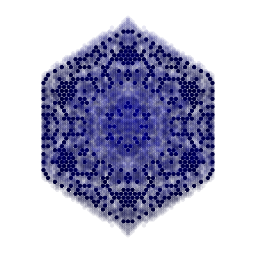
dnastore3.tcl

Produces the snowflake pattern shown at the top of this page.

dnastore4.tcl

A shell that forms and remains constant after a few simulation steps.

The structure of the script dnastore2.tcl, through twenty generations.

Using the DNA GUI window

The image below shows the GUI window for DNA as of version 3.3 (subject to change). In addition to the viewing window, there are two sliders on side and bottom that allow the view to be rotated. On the top is a row of buttons, whose functions are as follows:

Quit

Clean up and exit the application.

Load

Pop up a window showing script files that can be sourced for a new simulation.

Console

Pop up the console window, where commands affecting the simulation can be entered at the command-line prompt (see command-line syntax, below).

Rulesets

Pop up the ruleset display and edit window, which is shown in the figure below. Its function is described below.

Reset

Clear the window and all data in preparation for a new simulation.

Step

Advance one simulation step.

Cut view

Change the view between a solid form (Cut view off), and a cut view where only the Z=0 plane is solid, and the rest semi-transparent.

Following the menu buttons is a slider that contols the zoom factor of the view. Slide to the right to zoom in, and slide to the left to zoom out.

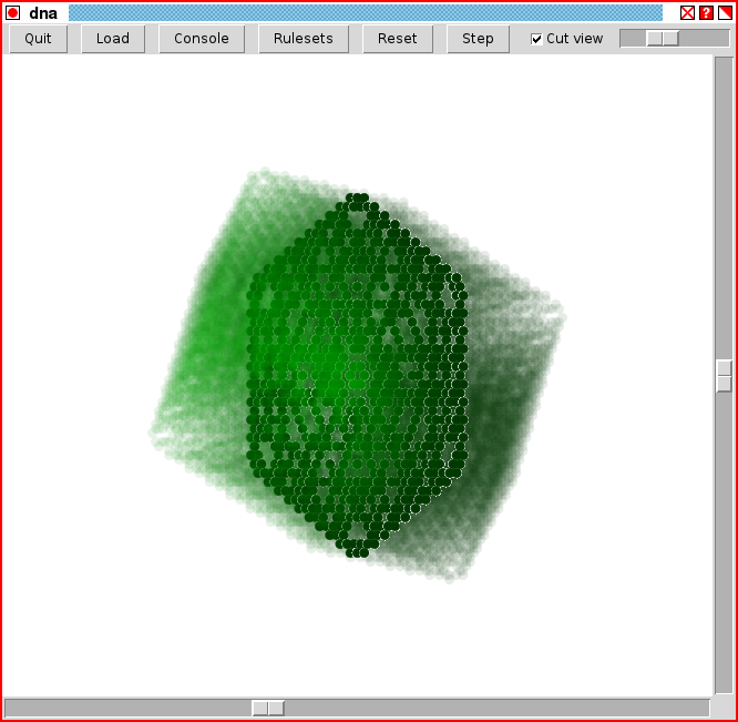
The DNA GUI window (DNA version 3.3).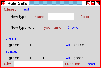

The ruleset display and edit window (DNA version 3.3).

Using the Ruleset display and edit window

The ruleset display and edit window provides full control over the contents of all rule sets in the simulation. On startup, the window will only contain the text "Ruleset: (none)". A new rule set can be added by loading a rule set from a file using the "Load" button in the main drawing window. Or a new rule can be created manually by clicking on the text "(none)", which brings up a pull-down menu with the option "New rule set...". By selecting "New rule set...", additional fields will be provided with an entry box to type a name for a new ruleset, and "Okay" and "Cancel" buttons. Type in a valid name for the rule set and type "Okay" to create an initially empty rule set. The new rule set will not be displayed initially, but once it is created, it will appear in the drop-down list of rule sets. From the drop-down list, it can be selected for display.

A rule set consists of a list of rules to apply when analyzing a coordinate due to the state of one of its neighbors being changed. A specific set of rules is applied depending on what type is present at the coordinate being checked. Every type, including space, can have a set of rules. To create a new set of rules for a particular type, select the type from the drop-down list after "Type name:", and then press the "New type rule" button. If no types have been loaded, then no types will be available in the drop-down menu.

To create a new type, write a name for the type in the "Name:" field, select a color in the "Color:" field, then press the "New type" button. Then the new type will be available for creating new type rule sets. Note that the type "space" needs to be created, but if it is not the first type created, then it will be generated automatically with default values when the first non-space type is created.

When a new set of rules for a type is first created using the "New type rule" button, a null rule (a rule with no effect) is created. This rule will not affect the simulation in any way, but it is expected that the user will replace the null rule with a functional one. Once created, the type rule set will have its type name written in blue on the left side of the window, followed by all of the rules to apply for that type, below it. Rules are applied in the order that they appear in this list. All rules are listed in the form:

type operator number ... => result

When a coordinate is being checked, the type of cell (or space) at that coordinate is recorded, and the number of each type of cell surrounding the cell being checked is recorded. The type of the cell being checked tells the automaton to use the ruleset for that type. The enumeration of neighboring types is checked against each rule condition, where a "condition" is defined as the triplet "type operator number". There may be any number of conditions which must all be satisfied in order for the rule to be satisfied.

A rule condition can use one of four legal operators: equal (=), greater than (>), less than (<), and not equal (~). If a condition is, for example, "space > 3", then the condition is satisfied if the cell being checked has more than three neighboring positions occupied by type space.

When the cursor passes over a rule in the rule set window, that rule will be highlighted. If the mouse button 1 (left button) is clicked while the rule is highlighted, then the rule function (shown at the bottom right corner of the window) will be applied at that rule position.

The rule function may be one of: Insert, Replace, Add, or Delete. All functions except delete require a valid rule to be written into the entry field "Rule:" on the bottom left. When the mouse left button is clicked over an existing rule, then the rule entered into this field will, respectively: be inserted before the existing rule, replace the existing rule, be added after the existing rule, or else the existing rule will be deleted. Using these rule functions, any rule set may be created manually.

It is also possible, and in some cases preferable, to enter rules at the command line, or write the command-line commands into a file that can be sourced with the "Load" button in the main window. The command-line commands do not provide any additional functionality to what is found in the ruleset display and edit window.

About DNA

Conway's game of "life" meets core wars. Conway's "life" is what is known as a "zero-player game". That is, one sets the starting conditions, and then it proceeds without interference. One important difference in "DNA" is that it is not necessarily a zero-player game, and lends itself to strategy games involving multiple players. Every cell is associated with a ruleset, and because cells can only be generated from neighboring cells, new cells acquire the rulesets of their neighbors when they are first generated. Therefore, clusters of cells can be seen as individual members of species, each behaving according to its own ruleset (or "DNA"). When two individuals are next to each other, a space cell that is between them may be claimed by both, or each may attempt to claim a cell belonging to the other. When this happens, a global set of fixed rules determines the winner. In this way, one individual can alter or destroy another, a combat scenario reminiscent of the old mainframe computer game "core wars".

The basic design of DNA comprises:

1. A virtual three-dimensional dense-packed hexagonal array grid for the automaton space (see below; this is not explicitly represented in memory).
   
   
2. A list of "cell" records. Each cell record represents something (that is not space) at a point in space. The individual record contains:
   
   
   • a position (x, y, z) which represents a euclidean- space mapping of the hexagonal array.
   • pointer to a table which is the type's "DNA" (see below). This table is shared by all records belonging to an "individual".
   • pointer to a "type" record
   
   
   The record is placed into a hash table by a hash of the position, so that any cell can be looked up by position. Note that the hashing of position avoids the necessity of maintaining a complete representation of 3-space in memory, so vast spaces can be simulated very quickly, if there are few cells changing within that space at each step.
   
   
3. Each table (the cell's DNA) contains:
   A prioritized list of condition:action pairs, where the condition includes a type (self), a list of conditions (neighboring cell type and number of neighbors that must have that cell type), and a result (what type the cell changes to given a match to the condition). That is, each entry has

   type operator number [type operator number ...] result

   where type is any valid type, operator is one of:
   
   

   "="

   there are exactly number neighboring cells of type

   "~"

   there are not exactly number neighboring cells of type

   "<"

   there are less than number neighboring cells of type

   ">"

   there are greater than number neighboring cells of type

   
   
   If there are multiple [type operator number] triplets, then all triplet rules must be satisfied for the overall rule to be satisfied (implied AND operation. OR operations can be made with multiple rules).

   If a type appears in more than one operator, then it implies that there is more than one distinct group of neighboring the cell. For example, the ruleset entry

   X = 3, X = 3, Y = 6

   indicates two clusters of 3 Xs separated by a cluster of 6 Ys. A single cluster of 6 Xs and a cluster of 6 Ys would not satisfy the condition. Note that clustering is not yet implemented in version 3.
   
   
4. Each type record contains:

   color used to render the type

5. An event stack for recording changes to be made, and an event hash table for recording positions that need to be checked on the next turn.

Simulation proceeds as follows:

1. Initial world has no records, no events, and nothing happens.
   
   
2. By Tcl command or in the Tk GUI, the user can create a DNA table. Then the user creates a cell at some point (preferably in the view window), gives it a type, and attaches the DNA table. Creating the cell generates a "create" event which is pushed on the event stack.
   
   
3. The simulator pulls the "create" event off the stack, and creates the new cell (actually, all events are "change" events; a "create" event changes a space cell into a cell of a non-space type).
   
   
4. The simulator sets a "recompute" event for each of the cell's 12 neighbors by setting a record in the check event table with the hash key being the cell position. There is then only one check recorded per position (except when more than one rule table wants to claim an open space, in which case the records are chained together in the same hash table record).
   
   
5. Loop through all create/change events.
   
   
6. Processing the contents of the check event table in order, the simulator grabs the first of the "recompute" events for the newly created cell's neighbor cell.
   
   
7. All of the cell's neighbors are enumerated and a table is generated containing a list of types that surround the cell, and how many cells of each type are present.
   
   
8. The DNA table, which is hashed by cell type, is searched for the record pertaining to the type of the cell being checked. This restricts the number of rules that have to be checked.
   
   
9. For each entry in the DNA table, the table of neighboring types is checked to see if it satisfies the conditions of the entry.
   
   
10. The first table entry for which all rules are satisfied is the "winner". If the resulting type for the rule is different from the cell type, then the simulator pushes a type change event record on the stack.
    
    
11. Loop through all remaining check events
    
    
12. Repeat from step (3) unless there are no pending change/ create events.
    
    

Check events create new change events and change events create new check events, so the cycle continues for as long as something in the simulation is changing. If the simulation becomes static, all processing stops.

Simulation speed decreases with increasing number of cell changes per step, and is independent of the size of the three dimensional space, or the total number of cells.

Command-line interface

DNA is compiled as a module extending the Tcl interpreter language, so that all manipulation of the contents and behavior of the automaton can be managed from the Tcl command line, with more complicated behavior (such as an interactive GUI) being built up from Tcl scripts. DNA adds a number of new commands to the Tcl interpreter language which are described below.

The command-line interface is designed so that everything in the simulation can be manipulated directly from the command line. There is no data storage format; simulation states are saved by dumping the current state as a set of Tcl commands, and the state is loaded by sourcing a command file. The command file that sets up a simulation can contain additional commands, such as setting simulation options or adjusting the view in the graphics window.

The following commands are reserved by the simulation for internal purposes and should not be called by the user:

start

start the application

tag command proc

tag a command with a callback procedure to be run whenever the command executes. This is usually used to update the GUI in response to commands entered on the command-line.

The following are user commands affecting the database:

step

step one simulation cycle

verbose value

set the level of diagnostic information printed. Diagnostic information can also be queried by command-line command. Values recognized are "1" (diagnostic simulation information) and "2" (diagnostic graphics information).

quit

Quit the application.

init

Reinitialize the simulation. Removes all cells, types, rules, and pending events.

init space

Delete all cells and pending events from the simulation, leaving existing types and rules intact.

cell

With no options, returns a list of {x y z} positions of each cell in the simulation.

cell {x y z}

Return a list of {type ruleset} values for the cell located at the position {x y z}.

cell {x y z} type ruleset

Declare a new cell or a cell change at location {x y z}. On the next step, the cell at that location will be created if it doesn't exist, and will have its type set to type and ruleset set to ruleset whether or not it previously existed.

pending

With no options, returns a list of {x y z} positions of each pending event in the simulation.

pending {x y z}

Return a list of {type ruleset} values for the pending event located at the position {x y z} Note that the use of "cell {x y z} type ruleset" generates a pending event; the command "pending" can only be used to list pending events.

type

With no options, returns a list of names of all known types.

type name

Return the {r g b a} component list defining the color of the type named name. Values range from 0.0 to 1.0.

type name {r g b a}

Create a new type named name with the color values r, g, b, and a, where all color values range between 0.0 and 1.0. If the type already exists, its values will be set to those given.

rule

With no options, returns a list of names of all known rule sets.

rule list name

Returns a list of types that are handled by the rule set named name.

rule list name type

Returns a list of rules, in order, for the type type in the rule set name. Each rule is a list of the form:

{result1 condition1 result2 condition2 ... }

Where resultN is the resulting type to change to when conditionN is satisfied. Each condition is a list of rules that must be simultaneously satisfied, in the form

{type1 operator1 value1 type2 operator2 value2 ... }

Where type1 is the type of a neighboring cell, operator1 is one of "=", "~", "<", or ">", and value1 is the number of neighboring cells of type type1 that are required to be present to satisfy the condition.

rule add name

Generates a new null rule set called name containing no rules.

rule add name type [index] rule_list

Append a new rule to the list of rules for type type in the rule set named name. The rule is a list of the same form as returned by the "rule list name type" command. Note that because rules are appended, a rule set can be built up by specifying individual entries in the form

rule add name type {type1 condition1}
rule add name type {type2 condition2}

in addition to being specified in a single list. If argument index is not present, then the rule is added at the end of the list of rules for the type. If index is present, then the rule is added after the rule number index, where the index of the first rule is zero.

rule insert name type index rule_list

This is the same as "rule add" with an index value, except that the index is mandatory and the rule is inserted before the rule number index. The rule_list may include multiple rules.

rule replace name type index rule_list

This is the same as "rule insert", except that the rule at index index is replaced with the rules in rule_list. Note that index refers to a single rule, but the single rule may be replaced by any number of rules in rule_list. If rule_list is a null list ("{}"), then the rule at index index is deleted.

The following are user commands affecting the graphic output:

redraw

refresh the graphics window

zplane on|off|value

When the zplane state is "on", the graphics window shows only a slice through Z=value. value defaults to zero if not specified in a "zplane" command. When the zplane state is "off", all Z values are displayed.

view [ax ay]

With no arguments, returns the current view as a list of two values. With two arguments, sets the viewing angles. The two arguments are the angle of rotation, in degrees, around the X axis and the Y axis, respectively. The default view is {0 0}.

zoom [value]

Sets the zoom factor for the view. The default zoom factor is 4.

The following are procedures (defined in the dna.tcl script):

save filename

Save the current simulation state as a command file named . Note that the current state cannot be recovered for viewing, but if the saved file is loaded, the simulation will continue with the next step. To load a saved file, use the Tcl command "source filename".

rate value

Set the number of steps for a "multistep" simulation. Typically this would be set to 1. Set to zero to stop a continuous simulation.

multistep

Run the number of simulation steps defined by "rate". Do not redraw until all steps have been computed.

simulate

Run continuously. The simulation will stop if "rate" is set to zero.

Code History

version 3.3:

July 24, 2012
Added ruleset button and window with the ability to display, create, and modify rulesets and individual rules.
Extended the "rule" command to allow a broader range of syntax. Eliminated the "delete" rule function in favor of "replace" with a null rule {}.

version 3.2:

July 22, 2012
Added sliders for view angle and zoom and cut view, with appropriate tag callbacks from the interpreter.

version 3.1:

July 20, 2012
Put DNA up on the opencircuitdesign website
Introduced revision numbering
More complete GUI with view selection and menu buttons, and file load dialog
Changed view format to (theta, phi) angles
Moved example files to subdirectory "configurations"

version 3.0:

July 18, 2012
Use tkcon.tcl console
OpenGL graphics rendering
Fix issues with off-grid items. "cell" command no longer accepts off-grid coordinates

version 2:

July 17, 2012
Optimized processing (string hash the Point3D) due to poor hashing performance of the Tcl array hash.
Added code to handle contention between conflicting rulesets.
Removed load/save data format file; data input works from the command-line, or by sourcing a command file.

version 1:

July 15, 2012
Changed the checking part of the event loop from a stack to a hash table. The event loop is now in two separate parts, one for changes, one for checks.
Added zplane cuts for better visualization
Added verbose levels for diagnostic feedback

version 0:

July 13, 2012
Initial implementation, largely coded but untested.

---

Back to my home page. . .

email:

---As always, Caveat end-user.

Last updated: March 15, 2013 at 2:27pm